Elementary transformations of matrices and their properties. Matrix algebra - elementary transformations of matrices Elementary transformations of the determinant of a matrix

The next three operations are called elementary transformations of matrix rows:

1) Multiplication i-th line matrices for the number λ ≠ 0:

which we will write in the form (i) → λ(i).

2) Permutation of two rows in a matrix, for example the i-th and k-th rows:

which we will write in the form (i) ↔ (k).

3) Adding to the i-th row of the matrix its k-th row with coefficient λ:

which we will write in the form (i) → (i) + λ(k).

Similar operations on matrix columns are called elementary column transformations.

Each elementary transformation of the rows or columns of a matrix has inverse elementary transformation, which turns the transformed matrix into the original one. For example, the inverse transformation for permuting two strings is to permutate the same strings.

Each elementary transformation of the rows (columns) of the matrix A can be interpreted as a multiplication of A on the left (right) by a matrix of a special type. This matrix is obtained if the same transformation is performed on identity matrix. Let's take a closer look at elementary string conversions.

Let matrix B be the result i-th multiplication rows of a matrix A of type m×n by the number λ ≠ 0. Then B = E i (λ)A, where the matrix E i (λ) is obtained from the identity matrix E of order m by multiplying its i-th row by the number λ.

Let the matrix B be obtained as a result of permutation of the i-th and k-th rows of the m×n type matrix A. Then B = F ik A, where the matrix F ik is obtained from the identity matrix E of order m by permuting its i-th and k-th rows.

Let matrix B be obtained by adding its kth row with coefficient λ to the i-th row of an m×n matrix A. Then B = G ik (λ)А, where the matrix G ik is obtained from the identity matrix E of order m by adding the k-th row with the coefficient λ to the i-th row, i.e. at the intersection of the i-th row and the k-th column of the matrix E, the zero element is replaced by the number λ.

Elementary transformations of the columns of matrix A are implemented in exactly the same way, but at the same time it is multiplied by matrices of a special type not on the left, but on the right.

Using algorithms that are based on elementary transformations of rows and columns, matrices can be transformed into different forms. One of the most important such algorithms forms the basis of the proof of the following theorem.

Theorem 10.1. Using elementary row transformations, any matrix can be reduced to stepped view.

◄ The proof of the theorem consists in constructing a specific algorithm for reducing the matrix to echelon form. This algorithm consists of repeatedly repeating in a certain order three operations associated with some current matrix element, which is selected based on its location in the matrix. At the first step of the algorithm, we select the upper left one as the current element of the matrix, i.e. [A] 11 .

1*. If the current element is zero, go to operation 2*. If it is not equal to zero, then the row in which the current element is located (the current row) is added with the appropriate coefficients to the rows located below, so that all matrix elements in the column under the current element become zero. For example, if the current element is [A] ij , then as the coefficient for the k-th row, k = i + 1, ... , we should take the number - [A] kj /[A] ij . We select a new current element, moving in the matrix one column to the right and one row down, and proceed to the next step, repeating operation 1*. If such a shift is not possible, i.e. the last column or row has been reached, we stop transforming.

2*. If the current element in some row of the matrix is zero, then we look through the matrix elements located in the column under the current element. If there are no non-zero ones among them, we proceed to operation 3*. Let in kth line there is a non-zero element below the current element. Swap the current and kth line and return to operation 1*.

3*. If the current element and all elements below it (in the same column) are equal to zero, we change the current element, moving one column to the right in the matrix. If such a shift is possible, i.e. the current element is not in the rightmost column of the matrix, then we repeat operation 1*. If we have already reached the right edge of the matrix and changing the current element is impossible, then the matrix has a stepped form, and we can stop transforming.

Since the matrix has finite dimensions, and in one step of the algorithm the position of the current element is shifted to the right by at least one column, the transformation process will end, and in no more than n steps (n is the number of columns in the matrix). This means that a moment will come when the matrix will have a stepped form.

Example 10.10. Let's transform the matrix to echelon form using elementary string transformations.

Using the algorithm from the proof of Theorem 10.1 and writing the matrices after completing its operations, we obtain

Elementary transformations are the following actions on the rows and columns of matrix A:

1) swapping two rows or columns of a matrix;

2) multiplying a row or column of a matrix by a number other than zero;

3) adding another row (column) to one row (column).

Theorem. Elementary transformations do not change the rank of the matrix, that is, if matrix B is obtained from matrix A by elementary transformations, then.

Proof. 1). When swapping two columns of a matrix, the maximum number of linearly independent columns does not change, and therefore its rank does not change.

2). Let the matrix B be obtained from the matrix A by multiplying the i-th row by the number t0 and r(A) =k. Obviously, any minor of matrix B that does not contain the ith row is equal to the corresponding minor of matrix A, and any minor of matrix B containing the ith row is equal to the corresponding minor of matrix A multiplied by number t. Consequently, the minor of order k of matrix B, corresponding to the basis minor of matrix A, will be non-zero, and all minors of order k+1 of matrix B, as well as all minors of order k+1 of matrix A, will be equal to zero. This means that r(B)=k=r(A).

3). Let matrix B be obtained from matrix A by adding the i-th row to the j-th row and r(A) = k. Minors of order k+1 of matrix B that do not contain the j-th row will be equal to the corresponding minors of matrix A, and therefore equal to zero. Minors of order k+1 of matrix B containing the ith and jth rows will be equal to the sum of two zero determinants. One of these determinants contains two identical rows (the j-th row contains the elements of the i-th row), and the second determinant is a minor of order k+1 of the matrix A and is therefore equal to zero. Minors of order k+1 of matrix B, containing the j-th row, but not containing the i-th row, will be equal to the sum of two minors of order k+1 of matrix A and therefore will also be equal to zero. Consequently, all minors of order k+1 of the matrix B are equal to 0 and r(B)k=r(A).

Let the matrix C be obtained from the matrix B by multiplying the i row by (-1). Then matrix A is obtained from matrix C by adding the i-th row to the j-th row and multiplying the i-th row by (-1). Therefore, as proved above, there will be r(A)r(C) =r(B). Thus, the inequalities r(B)r(A) and r(A)r(B) are simultaneously valid, which means that r(A) =r(B).

This property of elementary transformations is used in practice to calculate the rank of a matrix. To do this, using elementary transformations, we reduce this (non-zero) matrix A to a trapezoidal form, that is, to the form

B= ,

where elements for all i = 1,2,...,k; elements for all i > j and

i > k. Obviously, r(B) = k, that is, the rank of the matrix B is equal to the number of non-zero rows. This follows from the fact that the minor of order k of the matrix B, located at the intersection of the first k rows and columns, is a diagonal determinant and is equal to; and any minor of order k+1 of matrix B contains a zero row, which means it is equal to 0 (or, if k = n, there are no such minors at all).

Theorem. Any non-zero matrix A of dimension mn can be reduced to a trapezoidal shape using elementary transformations.

Proof. Since A0, then there is a matrix element
. By swapping the first and i-th rows, the first and j-th columns, we move the element to the upper left corner of the matrix and denote
. Then to the i-th row of the resulting matrix (i= 2,3, ...,m) we add the first row multiplied by the number . As a result of these elementary transformations, we obtain the matrix

A
.

If all elements
matrices A are equal to zero, then the theorem is proven. If there is an element
, then, by rearranging the second and i-th rows, the second and j-th columns of matrix A, we move the element in place of the element and denote
(If
, then we immediately denote
). Then to the i-th row of the resulting matrix (i= 3, ...,m) we add the second row multiplied by the number . As a result, we get the matrix

Continuing this process, in a finite number of steps we obtain matrix B, that is, we reduce matrix A to a trapezoidal shape.

Example. Let's calculate the rank of the matrix



. The arrows indicate the following elementary transformations: 1) the first and second lines were swapped; 2) added a third to the fourth line; 3) added the first line, multiplied by -2, to the third line, and divided the fourth line by 3; 4) divided the third line by 5 and swapped the third and fourth lines; 5) a second line was added to the third line, multiplied by -3, and a third was added to the fourth line. It can be seen that the matrix obtained from matrix A by the indicated elementary transformations has a trapezoidal shape with three non-zero rows. Therefore, r(A) = 3.

Elementary matrix transformations include:

1. Changing the order of rows (columns).

2. Discarding zero rows (columns).

3. Multiplying the elements of any row (column) by one number.

4. Adding to the elements of any row (column) the elements of another row (column), multiplied by one number.

Systems of linear algebraic equations (Basic concepts and definitions).

1. System m linear equations with n called unknowns system of equations of the form:

2.By decision system of equations (1) is called a collection of numbers x 1 , x 2 , … , x n , turning each equation of the system into an identity.

3. System of equations (1) is called joint, if it has at least one solution; if a system has no solutions, it is called non-joint.

4. System of equations (1) is called certain, if it has only one solution, and uncertain, if it has more than one solution.

5. As a result of elementary transformations, system (1) is transformed to a system equivalent to it (i.e., having the same set of solutions).

To elementary transformations systems of linear equations include:

1. Discarding null rows.

2. Changing the order of lines.

3. Adding to the elements of any row the elements of another row, multiplied by one number.

Methods for solving systems of linear equations.

1) Inverse matrix method (matrix method) for solving systems of n linear equations with n unknowns.

System n linear equations with n called unknowns system of equations of the form:

Let us write system (2) in matrix form; for this we introduce notation.

Coefficient matrix for variables:

X = is a matrix of variables.

B = is a matrix of free terms.

Then system (2) will take the form:

A× X = B– matrix equation.

Solving the equation, we get:

X = A -1 × B

Example:

; ;

1) │A│= 15 + 8 ‒18 ‒9 ‒12 + 20 = 4  0 matrix A -1 exists.

Ã =

4) A -1 = × Ã = ;

X = A -1 × B

Answer:

2) Cramer’s rule for solving systems of n – linear equations with n – unknowns.

Consider a system of 2 – x linear equations with 2 – unknowns:

Let's solve this system using the substitution method:

From the first equation it follows:

Substituting into the second equation, we get:

Substituting the value into the formula for, we get:

The determinant Δ is the determinant of the system matrix;

Δ x 1 - determinant of the variable x 1 ;

Δ x 2 - determinant of the variable x 2 ;

Formulas:

x 1 =;x 2 =;…,x n = ;Δ  0;

- are called Cramer's formulas.

When finding determinants of unknowns X 1 , X 2 ,…, X n the column of coefficients for the variable whose determinant is found is replaced with a column of free terms.

Example: Solve a system of equations using Cramer's method

Solution:

Let us first compose and calculate the main determinant of this system:

Since Δ ≠ 0, the system has a unique solution, which can be found using Cramer’s rule:

where Δ 1, Δ 2, Δ 3 are obtained from the determinant of Δ by replacing the 1st, 2nd or 3rd column, respectively, with the column of free terms.

Thus:

Gauss method for solving systems of linear equations.

Consider the system:

The extended matrix of system (1) is a matrix of the form:

Gauss method is a method of sequentially eliminating unknowns from the equations of the system, starting from the second equation through m- that equation.

In this case, by means of elementary transformations, the matrix of the system is reduced to triangular (if m = n and system determinant ≠ 0) or stepwise (if m< n ) form.

Then, starting from the last equation by number, all unknowns are found.

Gauss method algorithm:

1) Create an extended matrix of the system, including a column of free terms.

2) If A 11  0, then divide the first line by A 11 and multiply by (– a 21) and add the second line. Similarly reach m-that line:

Page 1 divide by A 11 and multiply by (– A m 1) and add m– that page

Moreover, from the equations, starting from the second to m– that is, the variable will be excluded x 1 .

3) At the 3rd step, the second line is used for similar elementary transformations of lines from 3rd to m- Tuyu. This will eliminate the variable x 2, starting from the 3rd line through m– thuyu, etc.

As a result of these transformations, the system will be reduced to a triangular or stepped shape (in the case of a triangular shape, there will be zeros under the main diagonal).

Reducing a system to a triangular or stepped shape is called direct Gaussian method, and finding unknowns from the resulting system is called in reverse.

Example:

Direct move. Let us present the extended matrix of the system

using elementary transformations to stepwise form. Let's rearrange the first and second rows of the matrix A b, we get the matrix:

Let's add the second row of the resulting matrix with the first, multiplied by (‒2), and its third row with the first row, multiplied by (‒7). Let's get the matrix

To the third row of the resulting matrix we add the second row, multiplied by (‒3), resulting in a step matrix

Thus, we have reduced this system of equations to a stepwise form:

Reverse move. Starting from the last equation of the resulting stepwise system of equations, we sequentially find the values of the unknowns:

The transformation matrix is used to calculate new coordinates of an object when it is transformed. By changing the values of the elements of the transformation matrix, any transformations can be applied to objects (for example: scaling, mirroring, rotating, moving, etc.). During any transformation, the parallelism of the lines of the object is maintained.

Coordinates in PDF are expressed in terms of two-dimensional space. A point (x, y) in space can be expressed in vector form . The constant third element of this vector (1) is needed to use the vector with 3x3 matrices in the calculations described below.

The transformation between two coordinate systems is represented as a 3x3 matrix and is written as follows:

Coordinate transformations are expressed as matrix multiplications:

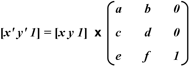
Since the last column does not have any influence on the calculation results, it does not take part in the calculations. Transformation coordinates are calculated using the following formulas:

Identity matrix

An identity matrix is one whose matrix values a And d equal 1 , and the rest are equal 0 . This matrix is used by default, since it does not lead to transformation. Therefore, the identity matrix is used as a basis.

Scaling

To increase or decrease the horizontal/vertical size of an object, change the value a or d accordingly, and apply the rest from the identity matrix.

For example: To double the size of an object horizontally, the value of a must be taken equal to 2, and the rest must be left as such in the identity matrix.

Reflection

To get a horizontal mirror image of an object, set the value a = -1, vertically d = -1. Changing both values is used to display both horizontally and vertically at the same time.

Incline

The tilt of the object vertically/horizontally is ensured by changing the values b And c respectively. Changing the value b/-b- tilt up/down, c/-c- right left.

For example: To tilt the object vertically up, set the value b = 1

We calculate the new coordinates of the object:

As a result, only the coordinate leads to the tilt of the object y, which increases by the value x.

Turn

Rotation is a combination of scaling and tilting, but to maintain the original proportions of an object, the transformation must be done with precise calculations using sines and cosines.

The rotation itself occurs counterclockwise, α specifies the rotation angle in degrees.

Moving

Moving is done by changing values e(horizontally) and f(vertically). Values are specified in pixels.

For example: Moving using a matrix is rarely used due to the fact that this operation can be done using other methods, for example, changing the position of an object in a tab.

Since the transformation matrix has only six elements that can be changed, it is visually displayed in PDF . Such a matrix can represent any linear transformation from one coordinate system to another. Transformation matrices are formed as follows:

Movements are indicated as , Where t x And t y— distances from the axis of the coordinate system horizontally and vertically, respectively.
Scaling is specified as . This scales the coordinates so that 1 unit in the horizontal and vertical dimensions in the new coordinate system is the same size as s x And s y units in the old coordinate system, respectively.
Rotations are made by the matrix , which corresponds to the rotation of the axes of the coordinate system by θ degrees counterclockwise.
The slope is indicated as , which corresponds to the axis tilt x at an angle α and axles y at an angle β .

The figure below shows examples of transformation. The directions of movement, angle of rotation and tilt shown in the figure correspond to the positive values of the matrix elements.

Matrix multiplications are not commutative—the order in which matrices are multiplied matters.

The table below shows the valid transformations and matrix values.

Original drawing	Transformed drawing	Matrix	Description
		1 0 0 2 0 0	Vertical scale. If the matrix value is greater than 1, the object expands, less than 1, it contracts.
		2 0 0 1 0 0	Horizontal scale. If the matrix value is greater than 1, the object expands, less than 1, it contracts.
		-1 0 0 1 0 0	Horizontal reflection.
		1 0 0 -1 0 0	Vertical reflection.
		1 1 0 1 0 0	Vertical tilt up.
		1 -1 0 1 0 0	Vertical tilt down.
		1 0 1 1 0 0	Horizontal tilt to the right.
		1 0 -1 1 0 0

Let us introduce the concept of an elementary matrix.

DEFINITION. A square matrix obtained from the identity matrix as a result of a non-special elementary transformation over the rows (columns) is called the elementary matrix corresponding to this transformation.

So, for example, the elementary matrices of the second order are the matrices

where A is any non-zero scalar.

The elementary matrix is obtained from the identity matrix E as a result of one of the following non-singular transformations:

1) multiplying a row (column) of the matrix E by a non-zero scalar;

2) adding (or subtracting) to any row (column) of matrix E another row (column) multiplied by a scalar.

Let us denote by the matrix obtained from the matrix E as a result of multiplying the row by a non-zero scalar A:

Let us denote by the matrix obtained from the matrix E as a result of adding (subtracting) to a row a row multiplied by A;

Let us denote the matrix obtained from the identity matrix E as a result of applying an elementary transformation over the rows; thus there is a matrix corresponding to the transformation

Let's consider some properties of elementary matrices.

PROPERTY 2.1. Any elementary matrix is invertible. The inverse of an elementary matrix is elementary.

Proof. Direct verification shows that for any non-zero scalar A. and arbitrary the equalities hold

Based on these equalities, we conclude that Property 2.1 holds.

PROPERTY 2.2. The product of elementary matrices is an invertible matrix.

This property follows directly from Property 2.1 and Corollary 2.3.

PROPERTY 2.3. If a non-singular rowwise elementary transformation transforms -matrix A into matrix B, then . The obscenity statement is also true.

Proof. If there is a multiplication of a string by a non-zero scalar A, then

If then

It is easy to check that the converse is also true.

PROPERTY 2.4. If matrix C is obtained from matrix A using a chain of non-singular rowwise elementary transformations, then. The converse is also true.

Proof. By property 2.3, the transformation transforms matrix A into matrix, transforms matrix into matrix, etc. Finally, transforms matrix into matrix Therefore, .

It is easy to check that the converse statement is also true. Conditions for matrix invertibility. To prove Theorem 2.8, the following three lemmas are needed.

LEMMA 2.4. A square matrix with a zero row (column) is irreversible.

Proof. Let A be a square matrix with zero row, B be any matrix, . Let be the zero row of matrix A; Then

i.e. the i-th row of matrix AB is zero. Therefore, matrix A is irreversible.

LEMMA 2.5. If the rows of a square matrix are linearly dependent, then the matrix is irreversible.

Proof. Let A be a square matrix with linearly dependent rows. Then there is a chain of non-singular rowwise elementary transformations that transform A into an echelon matrix; let such a chain. By property 2.4 of elementary matrices, the equality holds

where C is a matrix with a zero row.

Therefore, by Lemma 2.4, the matrix C is irreversible. On the other hand, if matrix A were invertible, then the product on the left in equality (1) would be an invertible matrix, like the product of invertible matrices (see Corollary 2.3), which is impossible. Therefore, matrix A is irreversible.