What is a Raid array and why does the average user need it? Creating a Raid Disk Array on Windows.
All modern motherboards are equipped with an integrated RAID controller, and top models even have several integrated RAID controllers. The extent to which integrated RAID controllers are in demand by home users is a separate question. In any case, a modern motherboard provides the user with the ability to create a RAID array of several disks. However, not every home user knows how to create a RAID array, what array level to choose, and generally has little idea of the pros and cons of using RAID arrays.
In this article, we will give brief recommendations on creating RAID arrays on home PCs and use a specific example to demonstrate how you can independently test the performance of a RAID array.
History of creation
The term “RAID array” first appeared in 1987, when American researchers Patterson, Gibson and Katz from the University of California Berkeley in their article “A Case for Redundant Arrays of Inexpensive Discs, RAID” described how In this way, you can combine several low-cost hard drives into one logical device so that the resulting capacity and performance of the system are increased, and the failure of individual drives does not lead to failure of the entire system.
More than 20 years have passed since this article was published, but the technology of building RAID arrays has not lost its relevance today. The only thing that has changed since then is the decoding of the RAID acronym. The fact is that initially RAID arrays were not built on cheap disks at all, so the word Inexpensive (inexpensive) was changed to Independent (independent), which was more true.
Operating principle
So, RAID is a redundant array of independent disks (Redundant Arrays of Independent Discs), which is tasked with ensuring fault tolerance and increasing performance. Fault tolerance is achieved through redundancy. That is, part of the disk space capacity is allocated for official purposes, becoming inaccessible to the user.
Increased performance of the disk subsystem is ensured by the simultaneous operation of several disks, and in this sense, the more disks in the array (up to a certain limit), the better.
The joint operation of disks in an array can be organized using either parallel or independent access. With parallel access, disk space is divided into blocks (strips) for recording data. Similarly, information to be written to disk is divided into the same blocks. When writing, individual blocks are written to different disks, and multiple blocks are written to different disks simultaneously, which leads to increased performance in write operations. The necessary information is also read in separate blocks simultaneously from several disks, which also increases performance in proportion to the number of disks in the array.
It should be noted that the parallel access model is implemented only if the size of the data write request is larger than the size of the block itself. Otherwise, parallel recording of several blocks is almost impossible. Let's imagine a situation where the size of an individual block is 8 KB, and the size of a request to write data is 64 KB. In this case, the source information is cut into eight blocks of 8 KB each. If you have a four-disk array, you can write four blocks, or 32 KB, at a time. Obviously, in the example considered, the write and read speeds will be four times higher than when using a single disk. This is only true for an ideal situation, but the request size is not always a multiple of the block size and the number of disks in the array.
If the size of the recorded data is less than the block size, then a fundamentally different model is implemented - independent access. Moreover, this model can also be used when the size of the data being written is larger than the size of one block. With independent access, all data from a single request is written to a separate disk, that is, the situation is identical to working with one disk. The advantage of the independent access model is that if several write (read) requests arrive simultaneously, they will all be executed on separate disks independently of each other. This situation is typical, for example, for servers.
In accordance with different types of access, there are different types of RAID arrays, which are usually characterized by RAID levels. In addition to the type of access, RAID levels differ in the way they accommodate and generate redundant information. Redundant information can either be placed on a dedicated disk or distributed among all disks. There are many ways to generate this information. The simplest of them is complete duplication (100 percent redundancy), or mirroring. In addition, error correction codes are used, as well as parity calculations.
RAID levels
Currently, there are several RAID levels that can be considered standardized - these are RAID 0, RAID 1, RAID 2, RAID 3, RAID 4, RAID 5 and RAID 6.
Various combinations of RAID levels are also used, which allows you to combine their advantages. Typically this is a combination of some kind of fault-tolerant level and a zero level used to improve performance (RAID 1+0, RAID 0+1, RAID 50).
Note that all modern RAID controllers support the JBOD (Just a Bench Of Disks) function, which is not intended for creating arrays - it provides the ability to connect individual disks to the RAID controller.
It should be noted that the RAID controllers integrated on motherboards for home PCs do not support all RAID levels. Dual-port RAID controllers only support levels 0 and 1, while RAID controllers with more ports (for example, the 6-port RAID controller integrated into the southbridge of the ICH9R/ICH10R chipset) also support levels 10 and 5.
In addition, if we talk about motherboards based on Intel chipsets, they also implement the Intel Matrix RAID function, which allows you to simultaneously create RAID matrices of several levels on several hard drives, allocating part of the disk space for each of them.
RAID 0
RAID level 0, strictly speaking, is not a redundant array and, accordingly, does not provide reliable data storage. Nevertheless, this level is actively used in cases where it is necessary to ensure high performance of the disk subsystem. When creating a RAID level 0 array, information is divided into blocks (sometimes these blocks are called stripes), which are written to separate disks, that is, a system with parallel access is created (if, of course, the block size allows it). By allowing simultaneous I/O from multiple disks, RAID 0 provides the fastest data transfer speeds and maximum disk space efficiency because no storage space is required for checksums. The implementation of this level is very simple. RAID 0 is mainly used in areas where fast transfer of large amounts of data is required.
RAID 1 (Mirrored disk)
RAID Level 1 is an array of two disks with 100 percent redundancy. That is, the data is simply completely duplicated (mirrored), due to which a very high level of reliability (as well as cost) is achieved. Note that to implement level 1, it is not necessary to first partition the disks and data into blocks. In the simplest case, two disks contain the same information and are one logical disk. If one disk fails, its functions are performed by another (which is absolutely transparent to the user). Restoring an array is performed by simple copying. In addition, this level doubles the speed of reading information, since this operation can be performed simultaneously from two disks. This information storage scheme is used mainly in cases where the cost of data security is much higher than the cost of implementing a storage system.
RAID 5
RAID 5 is a fault-tolerant disk array with distributed checksum storage. When recording, the data stream is divided into blocks (stripes) at the byte level and simultaneously written to all disks of the array in cyclic order.
Suppose the array contains n disks, and the stripe size d. For each portion of n–1 stripes, the checksum is calculated p.
Stripe d 1 recorded on the first disk, stripe d 2- on the second and so on up to the stripe dn–1, which is written to ( n–1)th disk. Next on n-disk checksum is written p n, and the process is repeated cyclically from the first disk on which the stripe is written dn.
Recording process (n–1) stripes and their checksum are produced simultaneously for all n disks.
The checksum is calculated using a bitwise exclusive-or (XOR) operation applied to the data blocks being written. So, if there is n hard drives, d- data block (stripe), then the checksum is calculated using the following formula:
pn=d1 d 2 ... d 1–1.
If any disk fails, the data on it can be restored using the control data and the data remaining on the working disks.
To illustrate, consider blocks of four bits each. Let there be only five disks for storing data and recording checksums. If there is a sequence of bits 1101 0011 1100 1011, divided into blocks of four bits, then to calculate the checksum it is necessary to perform the following bitwise operation:
1101 0011 1100 1011 = 1001.
Thus, the checksum written to the fifth disk is 1001.
If one of the disks, for example the fourth, fails, then the block d 4= 1100 will not be available when reading. However, its value can be easily restored using the checksum and the values of the remaining blocks using the same “exclusive OR” operation:
d4 = d1 d 2d 4p5.
In our example we get:
d4 = (1101) (0011) (1100) (1011) = 1001.
In the case of RAID 5, all disks in the array are the same size, but the total capacity of the disk subsystem available for writing becomes exactly one disk smaller. For example, if five disks are 100 GB in size, then the actual size of the array is 400 GB because 100 GB is allocated for control information.
RAID 5 can be built on three or more hard drives. As the number of hard drives in an array increases, its redundancy decreases.
RAID 5 has an independent access architecture, which allows multiple reads or writes to be performed simultaneously.
RAID 10
RAID level 10 is a combination of levels 0 and 1. The minimum requirement for this level is four drives. In a RAID 10 array of four drives, they are combined in pairs into level 0 arrays, and both of these arrays as logical drives are combined into a level 1 array. Another approach is also possible: initially the disks are combined into mirrored arrays of level 1, and then logical drives based on these arrays - into an array of level 0.
Intel Matrix RAID
The considered RAID arrays of levels 5 and 1 are rarely used at home, which is primarily due to the high cost of such solutions. Most often, for home PCs, a level 0 array on two disks is used. As we have already noted, RAID level 0 does not provide secure data storage, and therefore end users are faced with a choice: create a fast but unreliable RAID level 0 array or, doubling the cost of disk space, RAID- a level 1 array that provides reliable data storage, but does not provide significant performance benefits.
To solve this difficult problem, Intel developed Intel Matrix Storage Technology, which combines the benefits of Tier 0 and Tier 1 arrays on just two physical disks. And in order to emphasize that in this case we are not just talking about a RAID array, but about an array that combines both physical and logical disks, the word “matrix” is used in the name of the technology instead of the word “array”.
So, what is a two-disk RAID matrix using Intel Matrix Storage technology? The basic idea is that if the system has several hard drives and a motherboard with an Intel chipset that supports Intel Matrix Storage Technology, it is possible to divide the disk space into several parts, each of which will function as a separate RAID array.
Let's look at a simple example of a RAID matrix consisting of two disks of 120 GB each. Any of the disks can be divided into two logical disks, for example 40 and 80 GB. Next, two logical drives of the same size (for example, 40 GB each) can be combined into a RAID level 1 matrix, and the remaining logical drives into a RAID level 0 matrix.
In principle, using two physical disks, it is also possible to create just one or two RAID level 0 matrices, but it is impossible to obtain only level 1 matrices. That is, if the system has only two disks, then Intel Matrix Storage technology allows you to create the following types of RAID matrices:
- one level 0 matrix;
- two level 0 matrices;
- level 0 matrix and level 1 matrix.
If the system has three hard drives, the following types of RAID matrices can be created:
- one level 0 matrix;
- one level 5 matrix;
- two level 0 matrices;
- two level 5 matrices;
- level 0 matrix and level 5 matrix.
If the system has four hard drives, then it is additionally possible to create a RAID matrix of level 10, as well as combinations of level 10 and level 0 or 5.
From theory to practice
If we talk about home computers, the most popular and popular are RAID arrays of levels 0 and 1. The use of RAID arrays of three or more disks in home PCs is rather an exception to the rule. This is due to the fact that, on the one hand, the cost of RAID arrays increases in proportion to the number of disks involved in it, and on the other hand, for home computers, the capacity of the disk array is of primary importance, and not its performance and reliability.
Therefore, in the future we will consider RAID levels 0 and 1 based on only two disks. The objective of our research will be to compare the performance and functionality of RAID arrays of levels 0 and 1, created on the basis of several integrated RAID controllers, as well as to study the dependence of the speed characteristics of the RAID array on the stripe size.
The fact is that although theoretically, when using a RAID level 0 array, the read and write speed should double, in practice the increase in speed characteristics is much less modest and it varies for different RAID controllers. The same is true for a RAID level 1 array: despite the fact that theoretically the read speed should be doubled, in practice not everything is so smooth.
For our RAID controller comparison testing, we used the Gigabyte GA-EX58A-UD7 motherboard. This board is based on the Intel X58 Express chipset with the ICH10R southbridge, which has an integrated RAID controller for six SATA II ports, which supports the organization of RAID arrays of levels 0, 1, 10 and 5 with the Intel Matrix RAID function. In addition, the Gigabyte GA-EX58A-UD7 board integrates the GIGABYTE SATA2 RAID controller, which has two SATA II ports with the ability to organize RAID arrays of levels 0, 1 and JBOD.
Also on the GA-EX58A-UD7 board is an integrated SATA III controller Marvell 9128, on the basis of which two SATA III ports are implemented with the ability to organize RAID arrays of levels 0, 1 and JBOD.
Thus, the Gigabyte GA-EX58A-UD7 board has three separate RAID controllers, on the basis of which you can create RAID arrays of levels 0 and 1 and compare them with each other. Let us recall that the SATA III standard is backward compatible with the SATA II standard, therefore, based on the Marvell 9128 controller, which supports drives with the SATA III interface, you can also create RAID arrays using drives with the SATA II interface.
The testing stand had the following configuration:
- processor - Intel Core i7-965 Extreme Edition;
- motherboard - Gigabyte GA-EX58A-UD7;
- BIOS version - F2a;
- hard drives - two Western Digital WD1002FBYS drives, one Western Digital WD3200AAKS drive;
- integrated RAID controllers:
- ICH10R,
- GIGABYTE SATA2,
- Marvell 9128;
- memory - DDR3-1066;
- memory capacity - 3 GB (three modules of 1024 MB each);
- memory operating mode - DDR3-1333, three-channel operating mode;
- video card - Gigabyte GeForce GTS295;
- power supply - Tagan 1300W.
Testing was carried out under the Microsoft Windows 7 Ultimate (32-bit) operating system. The operating system was installed on a Western Digital WD3200AAKS drive, which was connected to the port of the SATA II controller integrated into the ICH10R south bridge. The RAID array was assembled on two WD1002FBYS drives with a SATA II interface.
To measure the speed characteristics of the created RAID arrays, we used the IOmeter utility, which is the industry standard for measuring the performance of disk systems.
IOmeter utility
Since we intended this article as a kind of user guide for creating and testing RAID arrays, it would be logical to start with a description of the IOmeter (Input/Output meter) utility, which, as we have already noted, is a kind of industry standard for measuring the performance of disk systems. This utility is free and can be downloaded from http://www.iometer.org.
The IOmeter utility is a synthetic test and allows you to work with hard drives that are not partitioned into logical partitions, so you can test drives regardless of the file structure and reduce the influence of the operating system to zero.
When testing, it is possible to create a specific access model, or “pattern,” which allows you to specify the execution of specific operations by the hard drive. If you create a specific access model, you are allowed to change the following parameters:
- size of the data transfer request;
- random/sequential distribution (in%);
- distribution of read/write operations (in%);
- The number of individual I/O operations running in parallel.
The IOmeter utility does not require installation on a computer and consists of two parts: IOmeter itself and Dynamo.
IOmeter is the controlling part of the program with a user graphical interface that allows you to make all the necessary settings. Dynamo is a load generator that has no interface. Each time you run IOmeter.exe, the Dynamo.exe load generator automatically starts.
To start working with the IOmeter program, just run the IOmeter.exe file. This opens the main window of the IOmeter program (Fig. 1).

Rice. 1. Main window of the IOmeter program
It should be noted that the IOmeter utility allows you to test not only local disk systems (DAS), but also network-attached storage devices (NAS). For example, it can be used to test the performance of a server's disk subsystem (file server) using several network clients. Therefore, some of the bookmarks and tools in the IOmeter utility window relate specifically to the program’s network settings. It is clear that when testing disks and RAID arrays we will not need these program capabilities, and therefore we will not explain the purpose of all tabs and tools.
So, when you start the IOmeter program, a tree structure of all running load generators (Dynamo instances) will be displayed on the left side of the main window (in the Topology window). Each running Dynamo load generator instance is called a manager. Additionally, the IOmeter program is multi-threaded and each individual thread running on a Dynamo load generator instance is called a Worker. The number of running Workers always corresponds to the number of logical processor cores.
In our example, we use only one computer with a quad-core processor that supports Hyper-Threading technology, so only one manager (one instance of Dynamo) and eight (according to the number of logical processor cores) Workers are launched.
Actually, to test disks in this window there is no need to change or add anything.
If you select the name of the computer with the mouse in the tree structure of running Dynamo instances, then in the window Target on the tab Disk Target All disks, disk arrays and other drives (including network drives) installed on the computer will be displayed. These are the drives that IOmeter can work with. Media may be marked yellow or blue. Logical partitions of media are marked in yellow, and physical devices without logical partitions created on them are marked in blue. A logical section may or may not be crossed out. The fact is that in order for the program to work with a logical partition, it must first be prepared by creating a special file on it, equal in size to the capacity of the entire logical partition. If the logical partition is crossed out, this means that the section is not yet prepared for testing (it will be prepared automatically at the first stage of testing), but if the section is not crossed out, this means that a file has already been created on the logical partition, completely ready for testing .
Note that, despite the supported ability to work with logical partitions, it is optimal to test drives that are not partitioned into logical partitions. You can delete a logical disk partition very simply - through a snap-in Disk Management. To access it, just right-click on the icon Computer on the desktop and select the item in the menu that opens Manage. In the window that opens Computer Management on the left side you need to select the item Storage, and in it - Disk Management. After that, on the right side of the window Computer Management All connected drives will be displayed. By right-clicking on the desired drive and selecting the item in the menu that opens Delete Volume..., you can delete a logical partition on a physical disk. Let us remind you that when you delete a logical partition from a disk, all information on it is deleted without the possibility of recovery.
In general, using the IOmeter utility you can only test blank disks or disk arrays. That is, you cannot test a disk or disk array on which the operating system is installed.
So, let's return to the description of the IOmeter utility. In the window Target on the tab Disk Target you must select the disk (or disk array) that will be tested. Next you need to open the tab Access Specifications(Fig. 2), on which it will be possible to determine the testing scenario.

Rice. 2. Access Specifications tab of the IOmeter utility
In the window Global Access Specifications There is a list of predefined test scripts that can be assigned to the boot manager. However, we won’t need these scripts, so all of them can be selected and deleted (there is a button for this Delete). After that, click on the button New to create a new test script. In the window that opens Edit Access Specification You can define the boot scenario for a disk or RAID array.
Suppose we want to find out the dependence of the speed of sequential (linear) reading and writing on the size of the data transfer request block. To do this, we need to generate a sequence of boot scripts in sequential read mode at different block sizes, and then a sequence of boot scripts in sequential write mode at different block sizes. Typically, block sizes are chosen as a series, each member of which is twice the size of the previous one, and the first member of this series is 512 bytes. That is, the block sizes are as follows: 512 bytes, 1, 2, 4, 8, 16, 32, 64, 128, 256, 512 KB, 1 MB. There is no point in making the block size larger than 1 MB for sequential operations, since with such large data block sizes the speed of sequential operations does not change.
So, let's create a loading script in sequential reading mode for a block of 512 bytes.
In field Name window Edit Access Specification enter the name of the loading script. For example, Sequential_Read_512. Next in the field Transfer Request Size set the data block size to 512 bytes. Slider Percent Random/Sequential Distribution(the percentage ratio between sequential and selective operations) we shift all the way to the left so that all our operations are only sequential. Well, the slider , which sets the percentage ratio between read and write operations, is shifted all the way to the right so that all our operations are read only. Other parameters in the window Edit Access Specification no need to change (Fig. 3).

Rice. 3. Edit Access Specification Window to Create a Sequential Read Load Script
with a data block size of 512 bytes
Click on the button Ok, and the first script we created will appear in the window Global Access Specifications on the tab Access Specifications IOmeter utilities.
Similarly, you need to create scripts for the remaining data blocks, however, to make your work easier, it is easier not to create the script anew each time by clicking the button New, and having selected the last created scenario, press the button Edit Copy(edit copy). After this the window will open again Edit Access Specification with the settings of our last created script. It will be enough to change only the name and size of the block. Having completed a similar procedure for all other block sizes, you can begin to create scripts for sequential recording, which is done in exactly the same way, except that the slider Percent Read/Write Distribution, which sets the percentage ratio between read and write operations, must be moved all the way to the left.
Similarly, you can create scripts for selective writing and reading.
After all the scripts are ready, they need to be assigned to the download manager, that is, indicate which scripts will work with Dynamo.
To do this, we check again what is in the window Topology The name of the computer (that is, the load manager on the local PC) is highlighted, and not the individual Worker. This ensures that load scenarios will be assigned to all Workers at once. Next in the window Global Access Specifications select all the load scenarios we have created and press the button Add. All selected load scenarios will be added to the window (Fig. 4).

Rice. 4. Assigning the created load scenarios to the load manager
After this you need to go to the tab Test Setup(Fig. 5), where you can set the execution time of each script we created. To do this in a group Run Time set the execution time of the load scenario. It will be enough to set the time to 3 minutes.

Rice. 5. Setting the execution time of the load scenario
Moreover, in the field Test Description You must specify the name of the entire test. In principle, this tab has a lot of other settings, but they are not needed for our tasks.
After all the necessary settings have been made, it is recommended to save the created test by clicking on the button with the image of a floppy disk on the toolbar. The test is saved with the extension *.icf. Subsequently, you can use the created load scenario by running not the IOmeter.exe file, but the saved file with the *.icf extension.
Now you can start testing directly by clicking on the button with a flag. You will be asked to specify the name of the file containing the test results and select its location. Test results are saved in a CSV file, which can then be easily exported to Excel and, by setting a filter on the first column, select the desired data with test results.
During testing, intermediate results can be seen on the tab Result Display, and you can determine which load scenario they belong to on the tab Access Specifications. In the window Assigned Access Specification a running script appears in green, completed scripts in red, and unexecuted scripts in blue.
So, we looked at the basic techniques for working with the IOmeter utility, which will be required for testing individual disks or RAID arrays. Note that we have not talked about all the capabilities of the IOmeter utility, but a description of all its capabilities is beyond the scope of this article.
Creating a RAID array based on the GIGABYTE SATA2 controller
So, we begin creating a RAID array based on two disks using the GIGABYTE SATA2 RAID controller integrated on the board. Of course, Gigabyte itself does not produce chips, and therefore under the GIGABYTE SATA2 chip is hidden a relabeled chip from another company. As you can find out from the driver INF file, we are talking about a JMicron JMB36x series controller.
Access to the controller setup menu is possible at the system boot stage, for which you need to press the Ctrl+G key combination when the corresponding inscription appears on the screen. Naturally, first in the BIOS settings you need to define the operating mode of the two SATA ports related to the GIGABYTE SATA2 controller as RAID (otherwise access to the RAID array configurator menu will be impossible).
The setup menu for the GIGABYTE SATA2 RAID controller is quite simple. As we have already noted, the controller is dual-port and allows you to create RAID arrays of level 0 or 1. Through the controller settings menu, you can delete or create a RAID array. When creating a RAID array, you can specify its name, select the array level (0 or 1), set the stripe size for RAID 0 (128, 84, 32, 16, 8 or 4K), and also determine the size of the array.
Once the array is created, then any changes to it are no longer possible. That is, you cannot subsequently change for the created array, for example, its level or stripe size. To do this, you first need to delete the array (with loss of data), and then create it again. Actually, this is not unique to the GIGABYTE SATA2 controller. The inability to change the parameters of created RAID arrays is a feature of all controllers, which follows from the very principle of implementing a RAID array.
Once an array based on the GIGABYTE SATA2 controller has been created, its current information can be viewed using the GIGABYTE RAID Configurer utility, which is installed automatically along with the driver.
Creating a RAID array based on the Marvell 9128 controller
Configuring the Marvell 9128 RAID controller is only possible through the BIOS settings of the Gigabyte GA-EX58A-UD7 board. In general, it must be said that the Marvell 9128 controller configurator menu is somewhat crude and can mislead inexperienced users. However, we will talk about these minor shortcomings a little later, but for now we will consider the main functionality of the Marvell 9128 controller.
So, although this controller supports SATA III drives, it is also fully compatible with SATA II drives.
The Marvell 9128 controller allows you to create a RAID array of levels 0 and 1 based on two disks. For a level 0 array, you can set the stripe size to 32 or 64 KB, and also specify the name of the array. In addition, there is an option such as Gigabyte Rounding, which needs explanation. Despite the name, which is similar to the name of the manufacturer, the Gigabyte Rounding function has nothing to do with it. Moreover, it is in no way connected with the RAID level 0 array, although in the controller settings it can be defined specifically for an array of this level. Actually, this is the first of those shortcomings in the Marvell 9128 controller configurator that we mentioned. The Gigabyte Rounding feature is defined only for RAID Level 1. It allows you to use two drives (for example, different manufacturers or different models) with slightly different capacities to create a RAID Level 1 array. The Gigabyte Rounding function precisely sets the difference in the sizes of the two disks used to create a RAID level 1 array. In the Marvell 9128 controller, the Gigabyte Rounding function allows you to set the difference in the sizes of the disks to 1 or 10 GB.
Another flaw in the Marvell 9128 controller configurator is that when creating a RAID level 1 array, the user has the ability to select the stripe size (32 or 64 KB). However, the concept of stripe is not defined at all for RAID level 1.
Creating a RAID array based on the controller integrated into the ICH10R
The RAID controller integrated into the ICH10R southbridge is the most common. As already noted, this RAID controller is 6-port and supports not only the creation of RAID 0 and RAID 1 arrays, but also RAID 5 and RAID 10.
Access to the controller setup menu is possible at the system boot stage, for which you need to press the key combination Ctrl + I when the corresponding inscription appears on the screen. Naturally, first in the BIOS settings you should define the operating mode of this controller as RAID (otherwise access to the RAID array configurator menu will be impossible).
The RAID controller setup menu is quite simple. Through the controller settings menu, you can delete or create a RAID array. When creating a RAID array, you can specify its name, select the array level (0, 1, 5 or 10), set the stripe size for RAID 0 (128, 84, 32, 16, 8 or 4K), and also determine the size of the array.
RAID performance comparison
To test RAID arrays using the IOmeter utility, we created sequential read, sequential write, selective read, and selective write load scenarios. The data block sizes in each load scenario were as follows: 512 bytes, 1, 2, 4, 8, 16, 32, 64, 128, 256, 512 KB, 1 MB.
On each of the RAID controllers, we created a RAID 0 array with all allowable stripe sizes and a RAID 1 array. In addition, in order to be able to evaluate the performance gain obtained from using a RAID array, we also tested a single disk on each of the RAID controllers.
So, let's look at the results of our testing.
GIGABYTE SATA2 Controller
First of all, let's look at the results of testing RAID arrays based on the GIGABYTE SATA2 controller (Fig. 6-13). In general, the controller turned out to be literally mysterious, and its performance was simply disappointing.
|
|
Rice. 6.Speed sequential |
Rice. 7.Speed sequential |
|
|
Rice. 12.Serial speed |
Rice. 13.Serial speed |


If you look at the speed characteristics of one disk (without a RAID array), the maximum sequential read speed is 102 MB/s, and the maximum sequential write speed is 107 MB/s.
When creating a RAID 0 array with a stripe size of 128 KB, the maximum sequential read and write speed increases to 125 MB/s, an increase of approximately 22%.
With stripe sizes of 64, 32, or 16 KB, the maximum sequential read speed is 130 MB/s, and the maximum sequential write speed is 141 MB/s. That is, with the specified stripe sizes, the maximum sequential read speed increases by 27%, and the maximum sequential write speed increases by 31%.
In fact, this is not enough for a level 0 array, and I would like the maximum speed of sequential operations to be higher.
With a stripe size of 8 KB, the maximum speed of sequential operations (reading and writing) remains approximately the same as with a stripe size of 64, 32 or 16 KB, however, there are obvious problems with selective reading. As the data block size increases up to 128 KB, the selective read speed (as it should) increases in proportion to the data block size. However, when the data block size is more than 128 KB, the selective read speed drops to almost zero (to approximately 0.1 MB/s).
With a stripe size of 4 KB, not only the selective read speed drops when the block size is more than 128 KB, but also the sequential read speed when the block size is more than 16 KB.
Using a RAID 1 array on a GIGABYTE SATA2 controller does not significantly change the sequential read speed (compared to a single drive), but the maximum sequential write speed is reduced to 75 MB/s. Recall that for a RAID 1 array, the read speed should increase, and the write speed should not decrease compared to the read and write speed of a single disk.
Based on the results of testing the GIGABYTE SATA2 controller, only one conclusion can be drawn. It makes sense to use this controller to create RAID 0 and RAID 1 arrays only if all other RAID controllers (Marvell 9128, ICH10R) are already used. Although it is quite difficult to imagine such a situation.
Marvell 9128 controller
The Marvell 9128 controller demonstrated much higher speed characteristics compared to the GIGABYTE SATA2 controller (Fig. 14-17). In fact, the differences appear even when the controller operates with one disk. If for the GIGABYTE SATA2 controller the maximum sequential read speed is 102 MB/s and is achieved with a data block size of 128 KB, then for the Marvell 9128 controller the maximum sequential read speed is 107 MB/s and is achieved with a data block size of 16 KB.
|
|
Rice. 18. Sequential speed If we talk about the RAID 0 array on the ICH10R controller, then the maximum sequential read and write speed does not depend on the stripe size and is 212 MB/s. Only the size of the data block at which the maximum sequential reading and writing speed is achieved depends on the stripe size. Test results show that for RAID 0 based on the ICH10R controller, it is optimal to use a 64 KB stripe. In this case, the maximum sequential read and write speed is achieved with a data block size of only 16 KB. So, to summarize, we once again emphasize that the RAID controller built into the ICH10R significantly exceeds all other integrated RAID controllers in performance. And given that it also has greater functionality, it is optimal to use this particular controller and simply forget about the existence of all the others (unless, of course, the system uses SATA III drives). |


Today we will talk about RAID arrays. Let's figure out what it is, why we need it, what it is like and how to use all this magnificence in practice.
So, in order: what is RAID array or simply RAID? This abbreviation stands for "Redundant Array of Independent Disks" or "redundant (backup) array of independent disks." To put it simply, RAID array this is a collection of physical disks combined into one logical disk.
Usually it happens the other way around - one physical disk is installed in the system unit, which we split into several logical ones. Here the situation is the opposite - several hard drives are first combined into one, and then the operating system is perceived as one. Those. The OS firmly believes that it physically only has one disk.
RAID arrays There are hardware and software.
Hardware RAID arrays are created before loading the OS using special utilities built into RAID controller- something like a BIOS. As a result of creating such RAID array already at the OS installation stage, the distribution kit “sees” one disk.
Software RAID arrays are created by OS tools. Those. During boot, the operating system “understands” that it has several physical disks, and only after the OS starts, through software, the disks are combined into arrays. Naturally, the operating system itself is not located on RAID array, since it is set before it is created.
"Why is all this needed?" - you ask? The answer is: to increase the speed of reading/writing data and/or increase fault tolerance and security.
"How RAID array can increase speed or secure data?" - to answer this question, consider the main types RAID arrays, how they are formed and what it gives as a result.
RAID-0. Also called "Stripe" or "Tape". Two or more hard drives are combined into one by sequential merging and summing up the volumes. Those. if we take two 500GB disks and create them RAID-0, the operating system will perceive this as one terabyte disk. At the same time, the read/write speed of this array will be twice as high as that of one disk, since, for example, if the database is physically located in this way on two disks, one user can read data from one disk, and another user can write to another disk at the same time. Whereas, if the database is located on one disk, the hard disk itself will perform read/write tasks of different users sequentially. RAID-0 will allow reading/writing in parallel. As a consequence, the more disks in the array RAID-0, the faster the array itself works. The dependence is directly proportional - the speed increases N times, where N is the number of disks in the array.
At the array RAID-0 there is only one drawback that outweighs all the advantages of using it - the complete lack of fault tolerance. If one of the physical disks of the array dies, the entire array dies. There's an old joke about this: "What does the '0' in the title mean? RAID-0? - the amount of information restored after the death of the array!"
RAID-1. Also called "Mirror" or "Mirror". Two or more hard drives are combined into one by parallel merging. Those. if we take two 500GB disks and create them RAID-1, the operating system will perceive this as one 500GB disk. In this case, the read/write speed of this array will be the same as that of one disk, since information is read/written to both disks simultaneously. RAID-1 does not provide a gain in speed, but provides greater fault tolerance, since in the event of the death of one of the hard drives, there is always a complete duplicate of information located on the second drive. It must be remembered that fault tolerance is provided only against the death of one of the array disks. If the data was deleted purposefully, it is deleted from all disks of the array simultaneously!
RAID-5. A more secure option for RAID-0. The volume of the array is calculated using the formula (N - 1) * DiskSize RAID-5 from three 500GB disks, we get an array of 1 terabyte. The essence of the array RAID-5 is that several disks are combined into RAID-0, and the last disk stores the so-called “checksum” - service information intended to restore one of the array disks in the event of its death. Array write speed RAID-5 somewhat lower, since time is spent calculating and writing the checksum to a separate disk, but the reading speed is the same as in RAID-0.
If one of the array disks RAID-5 dies, the read/write speed drops sharply, since all operations are accompanied by additional manipulations. Actually RAID-5 turns into RAID-0 and if recovery is not taken care of in a timely manner RAID array there is a significant risk of losing data completely.
With an array RAID-5 You can use the so-called Spare disk, i.e. spare. During stable operation RAID array This disk is idle and not used. However, in the event of a critical situation, restoration RAID array starts automatically - information from the damaged one is restored to the spare disk using checksums located on a separate disk.
RAID-5 is created from at least three disks and saves from single errors. In case of simultaneous occurrence of different errors on different disks RAID-5 doesn't save.
RAID-6- is an improved version of RAID-5. The essence is the same, only for checksums, not one, but two disks are used, and the checksums are calculated using different algorithms, which significantly increases the fault tolerance of everything RAID array generally. RAID-6 assembled from at least four disks. The formula for calculating the volume of an array looks like (N - 2) * DiskSize, where N is the number of disks in the array, and DiskSize is the size of each disk. Those. while creating RAID-6 from five 500GB disks, we get an array of 1.5 terabytes.
Write speed RAID-6 lower than RAID-5 by about 10-15%, which is due to additional time spent on calculating and writing checksums.
RAID-10- also sometimes called RAID 0+1 or RAID 1+0. It is a symbiosis of RAID-0 and RAID-1. The array is built from at least four disks: on the first RAID-0 channel, on the second RAID-0 to increase read/write speed, and between them in a RAID-1 mirror to increase fault tolerance. Thus, RAID-10 combines the advantages of the first two options - fast and fault-tolerant.
RAID-50- similarly, RAID-10 is a symbiosis of RAID-0 and RAID-5 - in fact, RAID-5 is built, only its constituent elements are not independent hard drives, but RAID-0 arrays. Thus, RAID-50 gives very good read/write speed and contains the stability and reliability of RAID-5.
RAID-60- the same idea: we actually have RAID-6, assembled from several RAID-0 arrays.
There are also other combined arrays RAID 5+1 And RAID 6+1- they look like RAID-50 And RAID-60 the only difference is that the basic elements of the array are not RAID-0 tapes, but RAID-1 mirrors.
How do you understand combined RAID arrays: RAID-10, RAID-50, RAID-60 and options RAID X+1 are direct descendants of the basic array types RAID-0, RAID-1, RAID-5 And RAID-6 and serve only to increase either read/write speed or increase fault tolerance, while carrying the functionality of basic, parent types RAID arrays.
If we move on to practice and talk about the use of certain RAID arrays in life, the logic is quite simple:
RAID-0 We do not use it in its pure form at all;
RAID-1 We use it where read/write speed is not particularly important, but fault tolerance is important - for example, on RAID-1 It’s good to install operating systems. In this case, no one except the OS accesses the disks, the speed of the hard disks themselves is quite sufficient for operation, fault tolerance is ensured;
RAID-5 We install it where speed and fault tolerance are needed, but there is not enough money to buy more hard drives or there is a need to restore arrays in case of damage without stopping work - spare Spare drives will help us here. Common Application RAID-5- data storage;
RAID-6 used where it is simply scary or there is a real threat of death of several disks in the array at once. In practice, it is quite rare, mainly among paranoid people;
RAID-10- used where it is necessary to work quickly and reliably. Also the main direction for use RAID-10 are file servers and database servers.
Again, if we simplify further, we come to the conclusion that where there is no large and voluminous work with files, it is quite enough RAID-1- operating system, AD, TS, mail, proxy, etc. Where serious work with files is required: RAID-5 or RAID-10.
The ideal solution for a database server is a machine with six physical disks, two of which are combined into a mirror RAID-1 and the OS is installed on it, and the remaining four are combined into RAID-10 for fast and reliable data processing.
If, after reading all of the above, you decide to install it on your servers RAID arrays, but don’t know how to do it and where to start - contact us! - we will help you select the necessary equipment, as well as carry out installation work for implementation RAID arrays.
Many users have heard about the concept of RAID disk arrays, but in practice few people imagine what it is. But as it turns out, there is nothing complicated here. Let's look at the essence of this term, as they say, on the fingers, based on the explanation of information for the average person.
What are RAID disk arrays?
First, let's look at the general interpretation offered by online publications. Disk arrays are entire information storage systems consisting of a combination of two or more hard drives that serve either to increase the speed of access to stored information or to duplicate it, for example, when saving backup copies.
In this combination, the number of hard drives in terms of installation theoretically has no restrictions. It all just depends on how many connections the motherboard supports. Actually, why are RAID disk arrays used? Here it is worth paying attention to the fact that in the direction of technology development (relative to hard drives), they have long frozen at one point (spindle speed 7200 rpm, cache size, etc.). The only exceptions in this regard are SSD models, but even they mainly only increase the volume. At the same time, progress in the production of processors or RAM strips is more noticeable. Thus, due to the use of RAID arrays, the performance gain when accessing hard drives is increased.
RAID disk arrays: types, purpose
As for the arrays themselves, they can be conditionally divided according to the numbering used (0, 1, 2, etc.). Each such number corresponds to the performance of one of the declared functions.
The main ones in this classification are disk arrays with numbers 0 and 1 (later it will be clear why), since they are the ones assigned the main tasks.

When creating arrays with multiple hard drives connected, you should initially use the BIOS settings, where the SATA configuration section is set to RAID. It is important to note that the connected drives must have absolutely identical parameters in terms of volume, interface, connection, cache, etc.
RAID 0 (Striping)
Zero disk arrays are essentially designed to speed up access to stored information (writing or reading). As a rule, they can have from two to four hard drives in combination.

But the main problem here is that when you delete information on one of the disks, it disappears on the others. Information is written in the form of blocks alternately on each disk, and the increase in performance is directly proportional to the number of hard drives (that is, four disks are twice as fast as two). But the loss of information is only due to the fact that the blocks can be located on different disks, although the user in the same “Explorer” sees the files in a normal display.
RAID 1
Disk arrays with a single designation belong to the Mirroring category and are used to save data by duplicating.

Roughly speaking, in this state of affairs, the user loses somewhat in productivity, but he can be sure that if data disappears from one partition, it will be saved in another.
RAID 2 and higher
Arrays numbered 2 and higher have dual purpose. On the one hand, they are designed to record information, on the other hand, they are used to correct errors.

In other words, disk arrays of this type combine the capabilities of RAID 0 and RAID 1, but are not particularly popular among computer scientists, although their operation is based on the use
What is better to use in practice?
Of course, if you plan to use resource-intensive programs on your computer, for example, modern games, it is better to use RAID 0 arrays. If you work with important information that needs to be saved in any way, you will have to turn to RAID 1 arrays. Due to the fact that the links with numbers from two and higher never became popular; their use is determined solely by the desire of the user. By the way, the use of zero arrays is also practical if the user often downloads multimedia files to the computer, say, movies or music with a high bitrate for the MP3 format or in the FLAC standard.
For the rest, you will have to rely on your own preferences and needs. The use of this or that array will depend on this. And, of course, when installing a bundle, it is better to give preference to SSD drives, since compared to conventional hard drives they already have higher write and read speeds. But they must be absolutely identical in their characteristics and parameters, otherwise the connected combination simply will not work. And this is precisely one of the most important conditions. So you will have to pay attention to this aspect.
Greetings to blog readers!
Today there will be another article on a computer topic, and it will be devoted to such a concept as Raid disk array- I’m sure this concept will mean absolutely nothing to many, and those who have already heard about it somewhere have no idea what it is. Let's figure it out together!
Without going into details of terminology, a Raid array is a kind of complex built from several hard drives, which allows you to more competently distribute functions between them. How do we usually place hard drives in a computer? We connect one hard drive to Sata, then another, then a third. And disks D, E, F and so on appear in our operating system. We can place some files on them or install Windows, but essentially these will be separate disks - if we take out one of them, we will not notice anything at all (if the OS was not installed on it) except that we will not have access to those recorded on them files. But there is another way - to combine these disks into a system, give them a certain algorithm for working together, as a result of which the reliability of information storage or the speed of their operation will significantly increase.
But before we can create this system, we need to know whether the motherboard supports Raid disk arrays. Many modern motherboards already have a built-in Raid controller, which allows you to combine hard drives. Supported array circuits are available in the descriptions for the motherboard. For example, let’s take the first ASRock P45R2000-WiFi board that caught my eye in Yandex Market.
Here, a description of the supported Raid arrays is displayed in the "Sata Disk Controllers" section.
In this example, we see that the Sata controller supports the creation of Raid arrays: 0, 1, 5, 10. What do these numbers mean? This is a designation for various types of arrays in which disks interact with each other according to different schemes, which are designed, as I already said, to either speed up their operation or increase reliability against data loss.
If the computer motherboard does not support Raid, then you can purchase a separate Raid controller in the form of a PCI card, which is inserted into the PCI slot on the motherboard and gives it the ability to create arrays of disks. For the controller to work after installing it, you will also need to install the raid driver, which either comes on the disk with this model, or can simply be downloaded from the Internet. It is best not to skimp on this device and buy from some well-known manufacturer, for example Asus, and with Intel chipsets.

I suspect that you still don’t have a good idea of what we’re talking about, so let’s take a closer look at each of the most popular types of Raid arrays to make everything more clear.
RAID 1 array
Raid 1 array is one of the most common and budget options that uses 2 hard drives. This array is designed to provide maximum protection for user data, because all files will be simultaneously copied to 2 hard drives. In order to create it, we take two hard drives of equal size, for example 500 GB each, and make the appropriate settings in the BIOS to create the array. After this, your system will see one hard drive measuring not 1 TB, but 500 GB, although physically two hard drives work - the calculation formula is given below. And all files will be simultaneously written to two disks, that is, the second will be a full backup copy of the first. As you understand, if one of the disks fails, you will not lose a single piece of your information, since you will have a second copy of this disk.

Also, the failure will not be noticed by the operating system, which will continue to work with the second disk - only a special program that monitors the functioning of the array will notify you of the problem. You just need to remove the faulty disk and connect the same one, only a working one - the system will automatically copy all the data from the remaining working disk to it and continue working.
The disk volume that the system will see is calculated here using the formula:
V = 1 x Vmin, where V is the total capacity and Vmin is the storage capacity of the smallest hard drive.
RAID 0 array
Another popular scheme, which is designed to increase not the reliability of storage, but, on the contrary, the speed of operation. It also consists of two HDDs, but in this case the OS already sees the full total volume of the two disks, i.e. if you combine 500 GB disks into Raid 0, the system will see one 1 TB disk. The speed of reading and writing increases due to the fact that blocks of files are written alternately to two disks - but at the same time, the fault tolerance of this system is minimal - if one of the disks fails, almost all files will be damaged and you will lose part of the data - the one that was written to broken disk. After this, you will have to restore the information at the service center.

The formula for calculating the total disk space visible to Windows is:
If, before reading this article, you weren’t really worried about the fault tolerance of your system, but would like to increase the speed of operation, then you can buy an additional hard drive and feel free to use this type. By and large, at home the vast majority of users do not store any super-important information, and some important files can be copied to a separate external hard drive.
Array Raid 10 (0+1)
As the name itself suggests, this type of array combines the properties of the previous two - it’s like two Raid 0 arrays combined into Raid 1. Four hard drives are used, information is written to two of them in blocks one by one, as was the case in Raid 0 , and for the other two, complete copies of the first two are created. The system is very reliable and at the same time quite fast, but very expensive to organize. To create, you need 4 HDDs, and the system will see the total volume using the formula:
That is, if we take 4 disks of 500 GB, then the system will see 1 disk of 1 TB in size.

This type, as well as the next one, is most often used in organizations, on server computers, where it is necessary to ensure both high speed of operation and maximum security against loss of information in case of unforeseen circumstances.
RAID 5 array
The Raid 5 array is the optimal combination of price, speed and reliability. In this array, a minimum of 3 HDDs can be used; the volume is calculated using a more complex formula:
V = N x Vmin – 1 x Vmin, where N is the number of hard drives.
So, let's say we have 3 disks of 500 GB each. The volume visible to the OS will be 1 TB.
The array's operation scheme is as follows: blocks of divided files are written to the first two disks (or three, depending on their number), and the checksum of the first two (or three) is written to the third (or fourth). Thus, if one of the disks fails, its contents can be easily restored using the checksum available on the last disk. The performance of such an array is lower than that of Raid 0, but is as reliable as Raid 1 or Raid 10 and at the same time cheaper than the latter, because You can save on the fourth hard drive.
The diagram below shows a Raid 5 layout of four HDDs.

There are also other modes - Raid 2,3, 4, 6, 30, etc., but they are largely derivative of those listed above.
How to install Raid disk array on Windows?
I hope you understand the theory. Now let's look at practice - inserting a PCI Raid controller into the PCI Raid slot and installing drivers, I think, will not be difficult for experienced PC users.
How can we now create an array of connected hard drives in the Windows Raid operating system?
It is best, of course, to do this when you have just purchased and connected clean hard drives without an installed OS. First, we restart the computer and go into the BIOS settings - here we need to find the SATA controllers to which our hard drives are connected and set them to RAID mode.

After that, save the settings and restart the PC. On a black screen, information will appear that you have Raid mode enabled and about the key with which you can access its settings. The example below asks you to press the "TAB" key.

Depending on the Raid controller model, it may be different. For example, "CNTRL+F"

We go to the configuration utility and click something like “Create array” or “Create Raid” in the menu - the labels may differ. Also, if the controller supports several Raid types, you will be asked to choose which one you want to create. In my example, only Raid 0 is available.

After this, we return back to the BIOS and in the boot order setting we see not several separate disks, but one in the form of an array.

That's all - RAID is configured and now the computer will treat your disks as one. This is how, for example, Raid will be visible when installing Windows.

I think you have already understood the benefits of using Raid. Finally, I will give a comparative table of measurements of disk writing and reading speeds separately or as part of Raid modes - the result, as they say, is obvious.

Greetings to all, dear readers of the blog site. I think many of you have at least once come across such an interesting expression on the Internet - “RAID array”. What it means and why the average user might need it, that’s what we’ll talk about today. It is a well-known fact that it is the slowest component in a PC, and is inferior to the processor and.
To compensate for the “innate” slowness where it is completely out of place (we are talking primarily about servers and high-performance PCs), they came up with the use of a so-called RAID disk array - a kind of “bundle” of several identical hard drives operating in parallel. This solution allows you to significantly increase the speed of operation coupled with reliability.
First of all, a RAID array allows you to provide high fault tolerance for the hard drives (HDD) of your computer by combining several hard drives into one logical element. Accordingly, to implement this technology you will need at least two hard drives. In addition, RAID is simply convenient, because all the information that previously had to be copied to backup sources (external hard drives) can now be left “as is”, because the risk of its complete loss is minimal and tends to zero, but not always, about this a little lower.
RAID translates roughly like this: a protected set of inexpensive disks. The name comes from the times when large hard drives were very expensive and it was cheaper to assemble one common array of smaller disks. The essence has not changed since then, in general, like the name, only now you can make just a giant storage out of several large HDDs, or make it so that one disk duplicates another. You can also combine both functions, thereby getting the advantages of one and the other.
All these arrays are under their own numbers, most likely you have heard about them - raid 0, 1...10, that is, arrays of different levels.
Types of RAID
Speed Raid 0
Raid 0 has nothing like reliability, because it only increases speed. You need at least 2 hard drives, and in this case the data will be “cut” and written to both disks at the same time. That is, you will have access to the full capacity of these disks, and theoretically this means that you get 2 times higher read/write speeds.

But let's imagine that one of these disks breaks down - in this case, the loss of ALL your data is inevitable. In other words, you will still have to make regular backups in order to be able to restore the information later. Typically 2 to 4 disks are used here.
Raid 1 or “mirror”
Reliability is not compromised here. You get the disk space and performance of only one hard drive, but you have double the reliability. One disk breaks - the information will be saved on the other.

The RAID 1 level array does not affect the speed, but the volume - here you have at your disposal only half of the total disk space, of which, by the way, in RAID 1 there can be 2, 4, etc., that is, an even number. In general, the main feature of a first-level raid is reliability.
Raid 10
Combines all the best of the previous types. I propose to look at how this works using the example of four HDDs. So, information is written in parallel on two disks, and this data is duplicated on two other disks.

The result is a 2-fold increase in access speed, but also the capacity of only two of the four disks in the array. But if any two disks fail, no data loss will occur.
Raid 5
This type of array is very similar to RAID 1 in its purpose, only now you need at least 3 disks, one of them will store the information necessary for recovery. For example, if such an array contains 6 HDDs, then only 5 of them will be used to record information.

Due to the fact that data is written to several hard drives at once, the reading speed is high, which is perfect for storing a large amount of data there. But, without an expensive raid controller, the speed will not be very high. God forbid one of the disks breaks - restoring information will take a lot of time.
Raid 6
This array can survive the failure of two hard drives at once. This means that to create such an array you will need at least four disks, despite the fact that the write speed will be even lower than that of RAID 5.

Please note that without a powerful raid controller, such an array (6) is unlikely to be assembled. If you only have 4 hard drives, it is better to build RAID 1.
How to create and configure a RAID array

RAID controller
A raid array can be made by connecting several HDDs to a computer motherboard that supports this technology. This means that such a motherboard has an integrated controller, which is usually built into the . But, the controller can also be external, which is connected via a PCI or PCI-E connector. Each controller, as a rule, has its own configuration software.
The raid can be organized both at the hardware level and at the software level; the latter option is the most common among home PCs. Users do not like the controller built into the motherboard because of its poor reliability. In addition, if the motherboard is damaged, data recovery will be very problematic. At the software level, the role of the controller is played, if something happens, you can easily transfer your raid array to another PC.
Hardware
How to make a RAID array? To do this you need:
- Get it somewhere with raid support (in case of hardware RAID);
- Buy at least two identical hard drives. It is better that they are identical not only in characteristics, but also of the same manufacturer and model, and connected to the mat. board using one .
- Transfer all data from your HDDs to other media, otherwise they will be destroyed during the raid creation process.
- Next, you will need to enable RAID support in the BIOS, but I can’t tell you how to do this in the case of your computer, due to the fact that everyone’s BIOS is different. Usually this parameter is called something like this: “SATA Configuration or Configure SATA as RAID”.
- Then restart your PC and a table with more detailed raid settings should appear. You may have to press the key combination "ctrl+i" during the POST procedure for this table to appear. For those who have an external controller, you will most likely need to press “F2”. In the table itself, click “Create Massive” and select the required array level.
After creating a raid array in the BIOS, you need to go to “disk management” in OS –10 and format the unallocated area - this is our array.
Program
To create a software RAID, you don't have to enable or disable anything in the BIOS. In fact, you don't even need raid support on your motherboard. As mentioned above, the technology is implemented using the PC’s central processor and Windows itself. Yep, you don't even need to install any third-party software. True, in this way you can only create a RAID of the first type, which is a “mirror”.

Right-click on “my computer” - “manage” - “disk management”. Then click on any of the hard drives intended for the raid (disk1 or disk2) and select “Create mirror volume.” In the next window, select a disk that will be a mirror of another hard drive, then assign a letter and format the final partition.

In this utility, mirrored volumes are highlighted in one color (red) and are designated by one letter. In this case, the files are copied to both volumes, once to one volume, and the same file is copied to the second volume. It is noteworthy that in the “my computer” window our array will be displayed as one section, the second section is hidden so as not to be an eyesore, because the same duplicate files are located there.

If a hard drive fails, the “Failed Redundancy” error will appear, while everything on the second partition will remain intact.
Let's summarize
RAID 5 is needed for a limited range of tasks, when a much larger number of HDDs (than 4 disks) are assembled into huge arrays. For most users, raid 1 is the best option. For example, if there are four disks with a capacity of 3 terabytes each, in RAID 1 in this case 6 terabytes of capacity are available. RAID 5 in this case will provide more space, however, the access speed will drop significantly. RAID 6 will give the same 6 terabytes, but even lower access speed, and will also require an expensive controller.
Let's add more RAID disks and you will see how everything changes. For example, let’s take eight disks of the same capacity (3 terabytes). In RAID 1, only 12 terabytes of space will be available for recording, half of the volume will be closed! RAID 5 in this example will give 21 terabytes of disk space + it will be possible to get data from any one damaged hard drive. RAID 6 will give 18 terabytes and data can be obtained from any two disks.
In general, RAID is not a cheap thing, but personally I would like to have at my disposal a RAID of the first level of 3 terabyte disks. There are even more sophisticated methods, like RAID 6 0, or “raid from raid arrays”, but this makes sense with a large number of HDDs, at least 8, 16 or 30 - you must agree, this goes far beyond the scope of ordinary “household” use and is used demand is mostly in servers.
Something like this, leave comments, add the site to bookmarks (for convenience), there will be many more interesting and useful things, and see you soon on the blog pages!