Excel selection from a drop-down list by condition. Creating a Dropdown List in Excel

When filling out a table in Excel, the data is often repeated. For example, you write the name of the product or the full name of the employee. Today we will talk about how to make a drop-down list in Excel so that you don’t constantly enter the same thing, but simply select the desired value.

There is the easiest way to cope with the task. You right-click on the cell under the data column to open the context menu. Here we look for the “Select from drop-down list” item. The same action can be easily performed using the combination Alt + down arrow.

That's just this method will not work if you need to make such an object in Excel in another cell and in 2-3, etc. before and after. If necessary, use the following option.

Traditional way

Select the area of the cells themselves from which you will create a drop-down list, then proceed:

Insert/Name/Assign (Excel 2003)

In the latest versions (2007, 2010, 2013, 2016) go to:

Formulas/Defined Names/Name Manager/New

Enter any name and tap OK.

Then select the cells (or several) where you plan to insert the list of specified fields. Go to the menu:

Data/Data Type/List

In the “Source” section, enter the previously written name, simply mark the range. You can copy the resulting cell to any place; it will already have a menu of specified table elements.

Additionally, you can stretch it to create a range. By the way, if the information in it changes, the list information will also change; it is dynamic.

How to make a drop-down list in Excel: using management methods

When you use this option, you insert a control that represents the data range itself. For this:

firstly, look for the “Developer” section (Excel 2007/2010), in other editions you activate it yourself through the “Customize Ribbon” parameters;

secondly, go to the section, click “Insert”;
thirdly, select “Field...” and click on the icon;
draw a rectangle;

right-click on it and click Format Object;

look for “Form…”, select the required boundaries;
mark the area where you want to set the serial number of the element in the list;
Click OK.

How to create a drop-down menu in Excel: using ActiveX elements

The steps are similar to those described above, but we are looking for “Field with ActiveX”.

The main differences here are that the ActiveX special element can be in 2 variants - debugging mode, which allows you to change parameters, and input mode, which only allows you to select information from it. You can change the mode using the key Design Mode In chapter Developer. Using this method, you can customize the color, font, and perform quick searches.

Additional features

IN Excel program It is possible to create a linked drop-down list. That is, when you select a value, you can select the parameters it needs in another column. For example, you choose a product, and you need to mark the unit of measurement, for example, gram, kilogram.

First of all, you should make a sign with the lists themselves, and then separate windows with the names of the products.

For the second, we activate the information check window, but in the “Source” item we write “=INDIRECT” and the address of the 1st cell. Everything worked out.

After this, so that the windows below are supplemented with the same properties, select the upper section and drag everything down with the mouse pressed. Ready.

How to make a drop-down list in Excel? As you can see, this is easy to do using any of the above methods. Just choose the most optimal one for yourself. And the choice will depend on the purpose of creation, purpose, area of use, amount of information and other things.

If you need to click on one of the cells in spreadsheet document Excel, a list with possible values was revealed, then you have come to the right place. In this article we will tell you about the most common and popular ways to do this. It doesn't take long. You don't need any special knowledge or skills. Only desire, attentiveness and strictly follow the written instructions. So, let's go!

Method 1. Standard.

First, you need to set the range of values that you want to see in your drop-down list. For example, let's talk about the cell "program". Let's create a list that should fall out of the cell.

Enter values for the drop-down list

If you have Excel 2003, then you need to follow these steps. Stand on the cell that you want to make as a drop-down list, select the menu Data – Verification.

Selecting the future list cell

In Excel 2007 and higher, this window is called up through the “ Data» -> « Data checking».

List in a cell in MS Excell 2010

You will see a verification dialog box where you need to enter range of values.

Specify the range of cells with list values

We set a specific type of input values, in our case we consider the element "List".

To specify the values of the drop-down list, there is a specific field - "source". Here you specify the range of cells from which the values for the drop-down list will be taken. This is done by clicking on the icon at the end of the line. Next, select a range of cells and press Enter.

This is the final result.

Ready cell with dropdown list

In order to in the field " Source" Do not constantly set a range of values. You can combine these values into one category, assign it a name and write this name in this column.

We indicate a specific list of values that should appear. Let's go and perform the following steps.

Step 1 – select menu – "Insert";
Step 2 - go to the menu "Name";
Step 3 - open the dialog box "Assign".

Create a constant with list values

If you have the English version then like this

Insert;
Name;
Define.

If you are working with the seventh office version or later of Excel 2007. Then the tab will help you "Formulas" - "Name Manager" (Namemanager), and select create. The choice of name is not limited in any way. You can write, for example "Review".

Creating a value range name in Excel 2010

Specify the name of the created range

Pay attention to this moment. The data source can be any named data range, for example, a price list.

In this case, when new items are added to the price catalog, they are automatically displayed in the drop-down menu. Also, one important point for such lists is the creation of related drop-down elements. In such cases. When the content changes in one element, the structure automatically changes and updates in the other.

Method 2 – Control element.

This method considers the option of adding a new object and linking it to a specific range in Excel. What steps need to be taken:

If you have an Excel version of 2007 or later, then select the Developer menu. If the version is early then View - Toolbars - Forms.

The list element is familiar to us from forms on websites. It is convenient to select ready-made values. For example, no one enters the month manually; it is taken from such a list. You can fill out a drop-down list in Excel using various tools. In this article we will look at each of them.

How to make a dropdown list in Excel

How to make a drop-down list in Excel 2010 or 2016 using one command on the toolbar? On the “Data” tab, in the “Working with Data” section, find the “Data Validation” button. Click on it and select the first item.

A window will open. In the “Options” tab, in the “Data type” drop-down section, select “List”.

A line will appear at the bottom to indicate sources.

You can provide information in different ways.

First let's assign a name. To do this, create such a table on any sheet.

Select it and right-click. Click on the “Assign a name” command.

Enter your name in the line above.

Call the “Data Check” window and in the “Source” field, specify the name by placing the “=” sign in front of it.

In any of the three cases you will see the desired element. Selecting a value from the dropdown Excel list happens with the mouse. Click on it and a list of specified data will appear.

You learned how to create a dropdown list in an Excel cell. But more can be done.

Dynamic Excel Data Substitution

If you add some value to the range of data that is inserted into the list, then no changes will occur in it until new addresses are manually specified. To link a range and an active element, you need to format the first one as a table. Create an array like this.

Select it and on the “Home” tab, select any table style.

Be sure to check the box below.

You will receive this design.

Create an active element as described above. For the source, enter the formula

INDIRECT("Table1[Cities]")

To find out the table name, go to the Design tab and look at it. You can change the name to any other.

The INDIRECT function creates a reference to a cell or range. Now your element in the cell is bound to the data array.

Let's try to increase the number of cities.

The reverse procedure - substituting data from a drop-down list into an Excel table - works very simply. In the cell where you want to insert the selected value from the table, enter the formula:

Cell_address

For example, if the list of data is in cell D1, then in the cell where the selected results will be displayed, enter the formula

How to remove (delete) a drop-down list in Excel

Open the drop-down list settings window and select "Any value" in the "Data type" section.

The unnecessary element will disappear.

Dependent Items

Sometimes in Excel there is a need to create several lists when one depends on the other. For example, each city has several addresses. When selecting the first one, we should receive only the addresses of the selected locality.

In this case, give each column a name. Select without the first cell (title) and right-click. Select "Name".

This will be the name of the city.

When naming St. Petersburg and Nizhny Novgorod, you will receive an error, since the name cannot contain spaces, underscores, special characters etc.

Therefore, we will rename these cities with an underscore.

We create the first element in cell A9 in the usual way.

And in the second we write the formula:

INDIRECT(A9)

You will first see an error message. Agree.

The problem is that there is no selected value. As soon as a city is selected in the first list, the second one will work.

How to Set Up Dependent Dropdown Lists in Excel with Search

You can use a dynamic data range for the second element. This is more convenient if the number of addresses grows.
Let's create a drop-down list of cities. The named range is highlighted in orange.

For the second list you need to enter the formula:

OFFSET($A$1,MATCH($E$6,$A:$A,0)-1,1,COUNTIF($A:$A,$E$6),1)

MATCH returns the number of the cell with the city selected in the first list (E6) in the specified area SA:$A.
COUNTIF counts the number of matches in a range with the value in the specified cell (E6).

We got linked dropdown lists in Excel with a match condition and a range search for it.

Multi-select

Often we need to get multiple values from a data set. You can display them in different cells, or you can combine them into one. In any case, a macro is needed.
Right-click on the sheet label at the bottom and select View Code.

The developer window will open. The following algorithm must be inserted into it.

Private Sub Worksheet_Change(ByVal Target As Range) On Error Resume Next If Not Intersect(Target, Range("C2:F2")) Is Nothing And Target.Cells.Count = 1 Then Application.EnableEvents = False If Len(Target.Offset (1, 0)) = 0 Then Target.Offset(1, 0) = Target Else Target.End(xlDown).Offset(1, 0) = Target End If Target.ClearContents Application.EnableEvents = True End If End Sub

Please note that in the line

If Not Intersect(Target, Range("E7")) Is Nothing And Target.Cells.Count = 1 Then

You should enter the address of the cell with the list. For us it will be E7.

Return to your Excel worksheet and create a list in cell E7.

When selected, the values will appear below it.

The following code will allow you to accumulate values in a cell.

Private Sub Worksheet_Change(ByVal Target As Range) On Error Resume Next If Not Intersect(Target, Range("E7")) Is Nothing And Target.Cells.Count = 1 Then Application.EnableEvents = False newVal = Target Application.Undo oldval = Target If Len(oldval)<>0 And oldval<>newVal Then Target = Target & "," & newVal Else Target = newVal End If If Len(newVal) = 0 Then Target.ClearContents Application.EnableEvents = True End If End Sub

As soon as you move the pointer to another cell, you will see a list of selected cities. To read this article.

We showed you how to add and change a drop-down list in an Excel cell. We hope this information helps you.

Have a great day!

A drop-down list refers to the content of several values in one cell. When the user clicks on the arrow on the right, a specific list appears. You can choose a specific one.

A very convenient Excel tool for checking entered data. The capabilities of drop-down lists allow you to increase the comfort of working with data: data substitution, display of data from another sheet or file, the presence of a search function and dependencies.

Creating a Dropdown List

Path: Data menu - Data Validation tool - Options tab. Data type – “List”.

You can enter the values from which the drop-down list will be composed in different ways:

Any of the options will give the same result.

Dropdown list in Excel with data substitution

You need to make a drop-down list with values from the dynamic range. If changes are made to the existing range (data is added or removed), they are automatically reflected in the drop-down list.

Let's test it. Here is our table with the list on one sheet:

Let’s add a new value “Christmas tree” to the table.

Now let’s remove the “birch” value.

The “smart table”, which easily “expands” and changes, helped us realize our plans.

Now let's make it possible to enter new values directly into the cell with this list. And the data was automatically added to the range.

When we enter a new name into an empty cell of the drop-down list, a message will appear: “Add the entered name baobab to the drop-down list?”

Click “Yes” and add another line with the value “baobab”.

Dropdown list in Excel with data from another sheet/file

When the values for the dropdown list are located on another sheet or in another workbook, standard way does not work. You can solve the problem using the INDIRECT function: it will generate the correct link to an external source of information.

We make active the cell where we want to place the drop-down list.
Open data verification options. In the “Source” field, enter the formula: =INDIRECT(“[List1.xlsx]Sheet1!$A$1:$A$9”).

The name of the file from which the information for the list is taken is enclosed in square brackets. This file must be open. If the book with the required values is located in another folder, you need to specify the full path.

How to make dependent dropdown lists

Let's take three named ranges:

This is a must. The above describes how to make a regular list a named range (using the “Name Manager”). Remember that the name cannot contain spaces or punctuation marks.

Let's create the first drop-down list, which will include the names of the ranges.

When you have placed the cursor in the “Source” field, go to the sheet and select the required cells one by one.

Now let's create a second dropdown list. It should reflect those words that correspond to the name selected in the first list. If “Trees”, then “hornbeam”, “oak”, etc. Enter in the “Source” field a function of the form =INDIRECT(E3). E3 – cell with the name of the first range.

Selecting multiple values from an Excel dropdown list

It happens when you need to select several items from a drop-down list at once. Let's consider ways to implement the task.

We create a standard list using the Data Validation tool. Add to source sheet ready macro. How to do this is described above. With its help, the selected values will be added to the right of the drop-down list.
To make the selected values appear below, we insert another handler code.
To display the selected values in one cell, separated by any punctuation mark, use the following module.

Private Sub Worksheet_Change(ByVal Target As Range)
On Error Resume Next
If Not Intersect(Target, Range("C2:C5")) Is Nothing And Target.Cells.Count = 1 Then
Application.EnableEvents = False
newVal = Target
Application.Undo
oldval = Target
If Len(oldval)<>0 And oldval<>newValThen
Target = Target & "," & newVal
Else
Target = newVal
End If
If Len(newVal) = 0 Then Target.ClearContents
Application.EnableEvents = True
End If
End Sub

Don’t forget to change the ranges to “your own”. We create lists in the classic way. And macros will do the rest of the work.

Dropdown list with search

When you enter the first letters on the keyboard, matching elements are highlighted. And these are not all the pleasant aspects of this tool. Here you can customize the visual presentation of information and specify two columns as a source at once.

The easiest way to complete this task is as follows. By pressing right button by cell under the data column call context menu. The field of interest here is Select from drop-down list. The same can be done by pressing the key combination Alt+Down Arrow.

However, this method will not work if you want to create a list in another cell that is not in the range and in more than one before or after. The following method will do this.

Standard method

Required select a range of cells, from which it will be created drop-down list, then Insert – Name – Assign(Excel 2003). In more new version(2007, 2010, 2013, 2016) go to the tab Formulas, where in the section Specific names find the button Name Manager.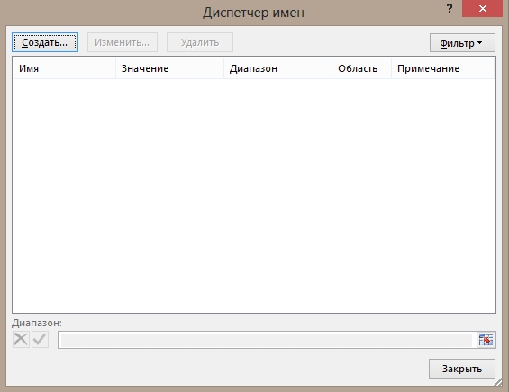

Press the button Create, enter a name, you can use any name, after which OK.

Select cells(or several) where you want to insert a drop-down list of required fields. From the menu, select Data – Data type – List. In field Source enter the previously created name, or you can simply specify the range, which will be equivalent.

Now the resulting cell can be copy anywhere on the sheet, it will contain a list of necessary table elements. You can also stretch it to get a range with drop-down lists.

An interesting point is that when the data in the range changes, the list based on it will also change, that is, it will dynamic.

Using the controls

The method is based on insert control called " combo box", which will represent a range of data.

Select a tab Developer(for Excel 2007/2010), in other versions you will need to activate this tab on the ribbon in parameters – Customize your feed.